Working with data in Excel often involves connecting information from different tables or datasets. This process, commonly referred to as data lookup or data merging, allows you to retrieve related values without manually searching through rows and columns. As datasets grow larger, manual searching becomes inefficient and prone to error, which is why Excel provides built-in functions to automate the process.
At a basic level, data lookup involves identifying a known value and using it to retrieve a corresponding value from another location. For example, if you have a list of customer names and a separate table containing customer IDs, you can use a lookup formula to match the name and return the correct ID. This method is widely used in business, finance, marketing, and data analysis tasks.
Understanding how lookup functions work is essential before moving into more advanced techniques. The most commonly used functions for this purpose are VLOOKUP and INDEX-MATCH. Each has its strengths and limitations, and choosing the right one depends on the structure and complexity of your data.
How Data Merging Works in Excel
Data merging is the process of combining information from two or more datasets based on a shared value. This shared value is often referred to as a key or identifier. In Excel, merging does not physically combine datasets; instead, it uses formulas to dynamically pull information from one table into another.
The concept is similar to searching in a directory. You start with a known value, such as a name or ID, and use it to locate related information, such as an address or phone number. Excel performs this task by scanning a specified range, identifying the position of the lookup value, and then returning the corresponding result.
This process typically involves three components:
- The lookup value, which is the known piece of information
- The lookup array, which is the range where Excel searches
- The return array, which is the range containing the desired result
By linking these components through a formula, Excel can automatically retrieve accurate data even as the dataset changes or grows.
Introduction to VLOOKUP
VLOOKUP is one of the earliest and most widely used lookup functions in Excel. It is designed to search for a value in the first column of a table and return a corresponding value from another column in the same row.
The function operates vertically, meaning it scans down a column until it finds a match. Once the match is found, it retrieves the value from a specified column to the right. This makes VLOOKUP simple to use, especially for beginners.
Despite its popularity, VLOOKUP has several limitations. It requires the lookup column to be positioned on the left side of the dataset. Additionally, it cannot return values from columns located to the left of the lookup column. Another limitation is the need to manually specify the column index number, which can lead to errors if the structure of the dataset changes.
Because of these constraints, VLOOKUP is best suited for simple tasks where the data structure remains fixed and predictable.
Limitations of VLOOKUP
Although VLOOKUP is useful, it becomes less practical as datasets become more complex. One of its main drawbacks is its inability to look in multiple directions. Since it only searches from left to right, any rearrangement of columns can break the formula.
Another issue is maintainability. If new columns are inserted or existing ones are moved, the column index number in the formula may no longer point to the correct data. This requires manual updates, which can be time-consuming and error-prone.
VLOOKUP also struggles with large datasets. While it can handle a reasonable amount of data, performance may decline when dealing with thousands of rows and multiple formulas.
These limitations have led many users to adopt more flexible alternatives, such as INDEX-MATCH.
Introduction to INDEX and MATCH
INDEX and MATCH are two separate functions that, when combined, provide a more powerful and adaptable lookup solution. Unlike VLOOKUP, this combination does not rely on fixed column positions, making it more resilient to changes in data structure.
The INDEX function is used to return a value from a specified position within a range. The MATCH function, on the other hand, is used to determine the position of a value within a range. When used together, MATCH identifies the position, and INDEX retrieves the value at that position.
This separation of responsibilities allows for greater flexibility and control. It also makes formulas easier to manage, especially in dynamic environments where data is frequently updated.
Understanding the INDEX Function
The INDEX function is designed to return a value based on its position within a dataset. Instead of searching for a value directly, it relies on row and column numbers to locate the desired result.
The function requires three main inputs: the data range, the row number, and optionally the column number. Once these inputs are provided, INDEX retrieves the value at the specified intersection.
This approach is particularly useful when you already know the position of the data you want. However, in most real-world scenarios, the position is not known in advance. This is where MATCH becomes essential.
Understanding the MATCH Function
MATCH is used to locate the position of a specific value within a range. It scans through the data and returns the relative position where the value is found.
One of the key features of MATCH is its ability to perform different types of searches. It can find exact matches, approximate matches, or values that meet certain conditions. For most lookup tasks, an exact match is used to ensure accuracy.
MATCH does not return the actual value; instead, it returns a number representing the position. This output is then used by INDEX to retrieve the corresponding data.
Combining INDEX and MATCH
When INDEX and MATCH are combined, they create a powerful lookup formula that overcomes many of the limitations of VLOOKUP. The MATCH function identifies the row position of the lookup value, and the INDEX function uses that position to return the desired result.
This combination allows you to separate the lookup logic from the return logic. As a result, you can search in one column and return values from another, regardless of their relative positions.
Another advantage is flexibility. Since the formula does not rely on fixed column numbers, it continues to work even if the dataset is rearranged. This makes it ideal for dynamic environments where data structures frequently change.
Advantages of INDEX-MATCH
INDEX-MATCH offers several benefits that make it a preferred choice for many Excel users. One of the most significant advantages is its ability to look in any direction. Unlike VLOOKUP, it is not restricted to searching from left to right.
Another benefit is improved performance with large datasets. INDEX-MATCH is generally more efficient, especially when working with complex spreadsheets containing multiple lookup formulas.
The formula is also easier to maintain. Since it does not depend on column index numbers, changes to the dataset do not require constant adjustments. This reduces the risk of errors and saves time in the long run.
When to Use INDEX-MATCH
INDEX-MATCH is particularly useful when working with datasets that contain unique identifiers. These identifiers serve as a reliable way to connect information across different tables.
Examples of such identifiers include customer IDs, product codes, and geographic labels. By using these identifiers, you can ensure that each lookup returns accurate and consistent results.
It is important to note that the lookup column should contain unique values whenever possible. If duplicates exist, the formula will return the first matching result, which may not always be correct.
Preparing Data for Lookup
Before creating any lookup formula, it is essential to organize your data properly. A well-structured dataset improves accuracy and makes formulas easier to build and maintain.
Start by ensuring that each column has a clear and descriptive header. These headers will later be used in advanced formulas, especially when working with multiple dimensions.
Next, identify the key column that will be used for matching. This column should contain consistent and preferably unique values. Any inconsistencies, such as extra spaces or spelling differences, should be corrected beforehand.
Finally, separate your datasets logically. Keep the reference data in one area and the main dataset in another. This separation helps prevent confusion and makes formulas easier to read.
Understanding Cell Referencing
Cell referencing plays a crucial role in Excel formulas. It determines how cell references behave when a formula is copied to other locations.
There are three main types of references. Absolute references lock both the row and column, ensuring that the reference does not change. Relative references adjust automatically based on the new position of the formula. Mixed references lock either the row or the column, providing a balance between flexibility and control.
Using the correct type of reference is essential for building scalable formulas. Incorrect referencing can lead to errors and inconsistent results, especially when formulas are copied across large ranges.
Importance of Referencing in Lookup Formulas
In lookup formulas, referencing ensures that the correct ranges are used throughout the calculation. For example, the lookup array should typically remain fixed, while the lookup value may change as the formula is copied down a column.
By using absolute references for fixed ranges and relative references for dynamic values, you can create formulas that adapt automatically without breaking.
This approach not only improves accuracy but also saves time, as you do not need to rewrite formulas for each row or column.
Setting Up the Worksheet
Creating a proper worksheet layout is the first step toward building effective lookup formulas. Begin by adding a new column where the results will be displayed. This column should have a header that clearly indicates the type of data it will contain.
Ensure that the reference dataset is easily accessible and clearly labeled. Keeping everything organized on the same worksheet can simplify the process, especially for beginners.
Once the layout is ready, you can begin constructing the lookup formula. Starting with a simple INDEX-MATCH formula helps build a strong foundation before moving on to more advanced techniques.
Building the Initial Lookup Formula
The first step in creating an INDEX-MATCH formula is selecting the return range. This is the column from which the final value will be retrieved.
Next, use the MATCH function to find the position of the lookup value within the lookup array. This position is then passed to the INDEX function, which retrieves the corresponding value from the return range.
By combining these steps, you create a formula that can dynamically locate and return data based on a specified input.
Transition to Advanced Techniques
While INDEX-MATCH is highly effective for one-dimensional lookups, it has limitations when dealing with more complex datasets that involve both rows and columns.
In such cases, a single MATCH function is not enough. You need a way to identify both the row and the column of the desired value. This is where the INDEX-MATCH-MATCH approach comes into play.
By adding a second MATCH function, you can extend the formula to work across two dimensions. This allows you to retrieve data from large and complex datasets with greater precision and flexibility.
In the next part, the focus will shift to building this advanced formula step by step, showing how to match both rows and columns effectively.
Building the INDEX-MATCH-MATCH Formula Step by Step
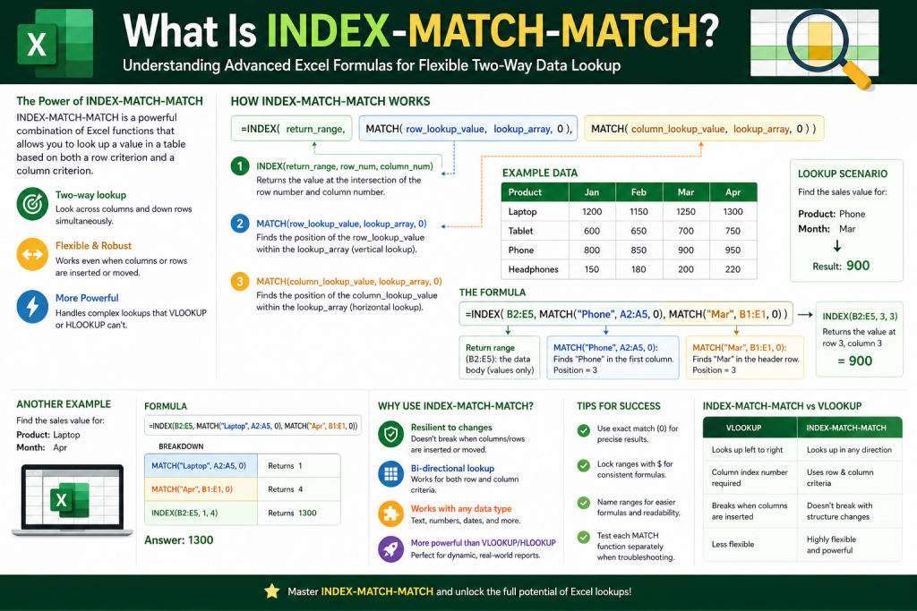
In the previous section, the foundation of lookup formulas was established using INDEX and MATCH. That combination allows Excel to retrieve data based on a single condition, typically matching a value in one column and returning a corresponding value from another. However, many real-world datasets are more complex and require retrieving data based on both row and column criteria.
This is where INDEX-MATCH-MATCH becomes essential. By introducing a second MATCH function, the formula gains the ability to locate both the correct row and the correct column. This creates a two-dimensional lookup system that can dynamically adapt to large datasets.
Understanding how to build this formula step by step is key to using it effectively.
Understanding Two-Dimensional Lookup
A standard INDEX-MATCH formula works in one direction. It finds a value in a column and returns a result from a corresponding row. This works well when you only need to match a single condition.
However, consider a dataset where:
- Rows represent items such as states or products
- Columns represent categories such as population, revenue, or codes
In this case, you are not just looking for a row match. You also need to identify which column contains the data you want. This requires two separate MATCH functions:
- One to locate the row
- One to locate the column
The INDEX function then uses both positions to return the correct value.
Structure of the INDEX-MATCH-MATCH Formula
The formula consists of three main components working together:
- INDEX provides the final value
- The first MATCH determines the row position
- The second MATCH determines the column position
The general structure looks like this:
INDEX(array, MATCH(row_lookup, row_range, 0), MATCH(column_lookup, column_range, 0))
Each part must be carefully defined to ensure the formula works correctly.
Preparing the Dataset
Before writing the formula, it is important to organize your data properly. A clean structure makes the formula easier to build and reduces the risk of errors.
Your dataset should include:
- A table containing the data you want to retrieve
- A column that contains unique row identifiers
- A row that contains unique column headers
For example, imagine a dataset where:
- Column A contains state names
- Row 1 contains headers such as population, area, and code
- The rest of the table contains the actual data
In addition, you may have another section where you want to retrieve specific values based on selected criteria.
Creating the Output Area
Start by setting up the area where the results will appear. This could be a separate table or a section within the same worksheet.
In this output area:
- One column will contain the row lookup values
- The top row will contain the column lookup values
This layout mirrors the structure of the main dataset and allows the formula to work in both directions.
Make sure the labels in this area match the source data exactly. Even small differences, such as extra spaces, can cause the formula to fail.
Step One: Defining the INDEX Array
The first step in building the formula is selecting the array for the INDEX function. This array should include all the values you want to retrieve.
It typically excludes row labels and column headers, focusing only on the data itself.
For example, if your dataset spans from B2 to E10, that range becomes your INDEX array.
It is important to lock this range using absolute references. This ensures that the array does not shift when the formula is copied to other cells.
Step Two: Writing the First MATCH Function
The first MATCH function is used to locate the correct row.
This function requires three inputs:
- The lookup value, which comes from the output area
- The range where Excel will search
- The match type, which is usually set to zero for an exact match
The lookup range should be the column that contains the row identifiers. This range should also be locked using absolute references.
The lookup value should use a mixed reference, where the column is locked but the row is allowed to change. This allows the formula to be copied down without breaking.
Step Three: Writing the Second MATCH Function
The second MATCH function is similar to the first but focuses on columns instead of rows.
It uses:
- A lookup value from the header row in the output area
- A lookup range consisting of the column headers in the dataset
- A match type of zero for exact matching
In this case, the reference should lock the row but allow the column to change. This enables the formula to be copied across multiple columns.
This step is what transforms the formula into a two-dimensional lookup tool.
Step Four: Combining All Components
Once both MATCH functions are written, they are inserted into the INDEX function as the row and column arguments.
At this point, the formula becomes fully functional. It can identify the correct row and column simultaneously and return the corresponding value.
When entered correctly, the formula should produce the expected result for the first cell in the output area.
Understanding How the Formula Works
To better understand the process, consider what happens behind the scenes:
- The first MATCH scans the row identifier column and finds the position of the lookup value
- The second MATCH scans the header row and finds the position of the desired column
- INDEX uses these two positions to locate the exact cell within the dataset
This coordinated process allows Excel to retrieve data accurately, even in large and complex tables.
Using Absolute and Mixed References Correctly
Referencing is critical in INDEX-MATCH-MATCH formulas. Without proper referencing, the formula may return incorrect results when copied.
The INDEX array should always use absolute references to remain fixed.
The first MATCH should lock the column but allow the row to change. This supports vertical copying.
The second MATCH should lock the row but allow the column to change. This supports horizontal copying.
By combining these reference types, the formula becomes fully dynamic.
Testing the Formula
After entering the formula, it is important to test it before copying it across the dataset.
Check the following:
- Does the result match the expected value
- Are there any error messages such as #N/A
- Do the lookup values exactly match the source data
If errors occur, verify that all ranges are correct and that references are properly locked.
Testing ensures that the formula is reliable before expanding it further.
Filling the Formula Down and Across
Once the formula is working correctly, it can be copied to other cells.
To fill the formula down:
- Drag the fill handle or use keyboard shortcuts
To fill the formula across:
- Drag horizontally across the header row
Because of the mixed referencing, the formula will adjust automatically and continue to produce correct results.
This ability to scale the formula is one of its greatest strengths.
Handling Errors in INDEX-MATCH-MATCH
Errors may occur for several reasons. The most common issue is the #N/A error, which indicates that a match could not be found.
Possible causes include:
- Mismatched text values
- Extra spaces in the data
- Incorrect ranges
To resolve these issues:
- Double-check the lookup values
- Ensure consistency in formatting
- Confirm that all ranges are correctly defined
In some cases, you may want to use error-handling functions to display a custom message instead of an error.
Working with Large Datasets
INDEX-MATCH-MATCH is especially useful when working with large datasets that contain multiple variables.
Instead of manually searching through rows and columns, the formula allows you to extract specific data points instantly.
This is particularly valuable in scenarios such as:
- Financial reporting
- Inventory tracking
- Data analysis
The formula reduces manual effort and improves accuracy, making it an essential tool for advanced Excel users.
Ensuring Unique Headers and Identifiers
For the formula to work correctly, both row identifiers and column headers must be unique.
If duplicate values exist:
- MATCH will return the first occurrence
- This may lead to incorrect results
To avoid this, ensure that:
- Each row identifier is distinct
- Each column header is clearly labeled and unique
This practice improves the reliability of your lookup formulas.
Practical Example of Two-Dimensional Lookup
Imagine a dataset containing sales data:
- Rows represent different products
- Columns represent different months
If you want to find the sales figure for a specific product in a specific month, INDEX-MATCH-MATCH can handle this easily.
By matching the product name and the month, the formula returns the exact value from the dataset.
This approach eliminates the need for manual searching and ensures consistent results.
Advantages of INDEX-MATCH-MATCH
This method provides several benefits:
- It allows lookups across both rows and columns
- It works with dynamic datasets
- It reduces dependency on fixed positions
- It improves efficiency in data retrieval
These advantages make it a powerful alternative to simpler lookup functions.
Transition to Advanced Applications
Now that the formula has been built and tested, it is ready for more advanced use cases.
In real-world scenarios, you may need to:
- Extract data from very large datasets
- Combine multiple lookup conditions
- Create dynamic reports
The next part will explore how to apply INDEX-MATCH-MATCH in practical situations, optimize performance, and use it alongside other Excel features to handle complex data tasks more effectively.
Applying INDEX-MATCH-MATCH in Real-World Scenarios
After understanding how to construct the INDEX-MATCH-MATCH formula, the next step is learning how to apply it effectively in practical situations. Real-world datasets are rarely simple. They often contain thousands of rows, multiple categories, and constantly changing structures. In such environments, a flexible and scalable lookup method becomes essential.
INDEX-MATCH-MATCH is particularly valuable when working with structured datasets that require both row-based and column-based matching. Instead of manually filtering or scanning through data, this formula allows you to retrieve precise information instantly. Whether you are working with financial data, sales reports, or operational metrics, the ability to perform two-dimensional lookups can significantly improve efficiency.
For example, in a sales dataset where products are listed in rows and months are listed in columns, this formula allows you to quickly find the sales figure for any product in any month. This eliminates repetitive manual work and ensures consistency in reporting.
Using INDEX-MATCH-MATCH for Dynamic Reporting
One of the most powerful applications of INDEX-MATCH-MATCH is in dynamic reporting. Reports often require pulling specific data points from large datasets based on changing criteria. Instead of rebuilding formulas each time, you can create a dynamic structure where inputs control the output.
In a dynamic report:
- Users can select a value such as a product, region, or time period
- The formula automatically updates to display the corresponding data
This setup is especially useful in dashboards, where decision-makers need quick access to specific insights. By linking input cells to the lookup formula, you create a system that responds instantly to changes.
This approach not only saves time but also reduces the risk of human error. Instead of manually searching for values, the formula ensures that the correct data is always retrieved.
Extracting Data from Large Datasets
Large datasets can be difficult to navigate manually. When dealing with thousands of rows and dozens of columns, finding a specific value can become time-consuming.
INDEX-MATCH-MATCH simplifies this process by allowing you to pinpoint exact values using defined criteria. Instead of scrolling through endless data, you simply provide the row and column identifiers, and the formula returns the result.
This is particularly useful in industries such as:
- Finance, where datasets may include multiple accounts and time periods
- Marketing, where performance metrics are tracked across campaigns
- Inventory management, where products are tracked across locations
By automating data retrieval, you can focus more on analysis and decision-making rather than data handling.
Combining INDEX-MATCH-MATCH with Other Functions
While INDEX-MATCH-MATCH is powerful on its own, it becomes even more effective when combined with other Excel functions. This allows you to handle more complex scenarios and improve the usability of your formulas.
For instance, you can combine it with error-handling functions to manage missing data. Instead of displaying an error message, the formula can return a custom message or a blank value. This improves the readability of your reports.
You can also integrate it with logical functions to create conditional lookups. For example, you might retrieve a value only if certain conditions are met. This adds another layer of flexibility to your data analysis.
By combining multiple functions, you can build robust solutions that handle a wide range of data challenges.
Improving Formula Efficiency
When working with large spreadsheets, efficiency becomes an important consideration. Complex formulas can slow down performance, especially when repeated across many cells.
To improve efficiency:
- Limit the size of your lookup ranges to only the necessary data
- Avoid using entire column references when not needed
- Keep your data clean and well-organized
Another useful approach is to use helper columns. These columns can simplify complex calculations and reduce the load on your main formula. While this may add extra steps, it can significantly improve performance in large datasets.
Efficient formulas not only run faster but are also easier to maintain and troubleshoot.
Avoiding Common Mistakes
Even experienced users can encounter issues when working with INDEX-MATCH-MATCH. Understanding common mistakes can help you avoid errors and build more reliable formulas.
One common issue is incorrect referencing. If ranges are not properly locked, the formula may shift when copied, leading to incorrect results. Ensuring the correct use of absolute and mixed references is essential.
Another issue is mismatched data. Differences in formatting, such as extra spaces or inconsistent capitalization, can prevent MATCH from finding the correct value. Cleaning your data before applying formulas is a crucial step.
Duplicate values can also cause problems. Since MATCH returns the first occurrence, duplicates may lead to unexpected results. Whenever possible, ensure that lookup values are unique.
By being aware of these issues, you can minimize errors and improve the accuracy of your work.
Scaling the Formula Across Worksheets
In many cases, your data may be spread across multiple worksheets. INDEX-MATCH-MATCH can be used across sheets just as easily as within a single sheet.
To do this, simply reference the appropriate sheet in your formula. This allows you to pull data from one sheet into another without duplicating information.
This approach is useful for:
- Consolidating data from different departments
- Creating summary reports
- Organizing large workbooks
By linking sheets together, you can maintain a clean and efficient structure while still accessing all necessary data.
Using INDEX-MATCH-MATCH for Data Analysis
Data analysis often requires comparing values across multiple dimensions. INDEX-MATCH-MATCH provides a reliable way to extract specific data points for analysis.
For example, you might want to compare sales performance across different regions and time periods. By using the formula, you can quickly retrieve the relevant values and perform further calculations.
This method allows you to:
- Identify trends
- Compare performance metrics
- Generate insights from large datasets
By automating data retrieval, you can spend more time analyzing results and less time searching for data.
Creating Flexible Data Models
A flexible data model is one that can adapt to changes without requiring constant updates. INDEX-MATCH-MATCH supports this by allowing you to build formulas that are not dependent on fixed positions.
If new rows or columns are added, the formula continues to work as long as the structure remains consistent. This makes it ideal for evolving datasets.
Flexible models are particularly important in business environments where data is constantly changing. By designing your formulas with adaptability in mind, you can reduce maintenance and improve long-term usability.
Comparing INDEX-MATCH-MATCH with Other Methods
There are several ways to perform lookups in Excel, including VLOOKUP, HLOOKUP, and newer functions like VLOOKUP. Each method has its own strengths.
Compared to these alternatives, INDEX-MATCH-MATCH offers:
- Greater flexibility in both directions
- Better compatibility with complex datasets
- More control over referencing
While newer functions may provide simpler syntax, INDEX-MATCH-MATCH remains a valuable tool, especially in environments where compatibility with older versions of Excel is required.
Understanding multiple methods allows you to choose the best approach for each situation.
Enhancing Data Accuracy
Accuracy is critical when working with data. Even small errors can lead to incorrect conclusions and poor decision-making.
INDEX-MATCH-MATCH helps improve accuracy by:
- Using exact match conditions
- Reducing manual data handling
- Providing consistent results
To further enhance accuracy, it is important to:
- Validate your data regularly
- Use consistent formatting
- Test formulas thoroughly
By combining these practices with reliable formulas, you can ensure high-quality data analysis.
Automating Repetitive Tasks
Many data tasks involve repetitive actions, such as retrieving values for multiple combinations of criteria. INDEX-MATCH-MATCH can automate these tasks, saving time and effort.
Once the formula is set up, it can be copied across rows and columns to handle large volumes of data. This eliminates the need for manual input and reduces the risk of errors.
Automation is especially valuable in tasks such as:
- Monthly reporting
- Performance tracking
- Data consolidation
By automating repetitive processes, you can focus on more strategic activities.
Adapting to Changing Data Structures
Data structures often change over time. New columns may be added, existing ones may be rearranged, and datasets may grow in size. These changes can create challenges when working with formulas that rely on fixed positions or static references. If a formula depends on a specific column index or a hardcoded structure, even a small modification in the dataset can lead to incorrect results or broken calculations. This is especially common in fast-paced environments where data is frequently updated, expanded, or reorganized to meet new requirements.
To manage these changes effectively, it is important to build formulas that are flexible and adaptable. Instead of relying on fixed column numbers, using dynamic lookup methods ensures that formulas continue to work even when the structure evolves. For example, when new columns are inserted, a well-designed lookup formula can still identify the correct data based on headers rather than position. This reduces the need for constant adjustments and minimizes the risk of errors.
Another important consideration is maintaining consistency in data formatting. When datasets grow, inconsistencies such as extra spaces, mismatched naming conventions, or duplicated headers can disrupt lookup operations. Regular data cleaning and validation help ensure that formulas continue to function as expected.
In addition, organizing data with clear headers and logical grouping makes it easier to adapt to structural changes. When datasets are well-structured, updating formulas becomes more straightforward, and the overall workflow remains efficient even as complexity increases.
INDEX-MATCH-MATCH is well-suited to handle these changes because it does not rely on fixed positions. As long as the lookup ranges are updated correctly, the formula continues to function.
This adaptability makes it a reliable choice for long-term projects and evolving datasets.
Best Practices for Using INDEX-MATCH-MATCH
To get the most out of this formula, it is important to follow best practices.
Keep your data organized and clearly labeled. Use consistent naming conventions for headers and identifiers. Avoid unnecessary complexity in your formulas, and break down large calculations into smaller steps when needed.
Regularly review and test your formulas to ensure they are working correctly. Document your work so that others can understand and maintain it.
By following these practices, you can build efficient and reliable solutions.
Conclusion
INDEX-MATCH-MATCH is a powerful and flexible method for retrieving data in Excel. By combining the strengths of INDEX and MATCH, it allows you to perform two-dimensional lookups that go beyond the capabilities of traditional functions.
Throughout this guide, the process of building and applying the formula has been explored in detail. From understanding basic lookup concepts to implementing advanced techniques, each step contributes to a deeper understanding of how Excel handles data.
This method is particularly useful in complex scenarios where both rows and columns must be matched. It provides accuracy, scalability, and adaptability, making it suitable for a wide range of applications.
While it may require more effort to learn compared to simpler functions, the benefits are significant. Once mastered, INDEX-MATCH-MATCH becomes an essential tool for data analysis, reporting, and decision-making.
By applying the concepts and best practices discussed, you can handle large datasets with confidence and efficiency.
Continue exploring the technologies and certification concepts that matter most to you.