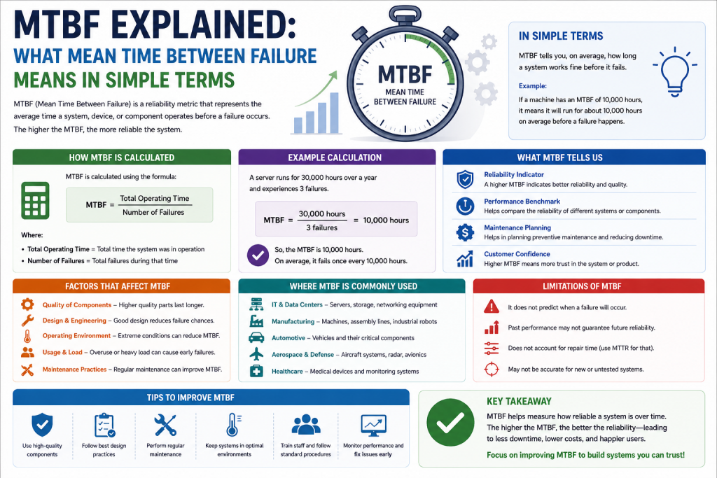
Mean Time Between Failure, commonly known as MTBF, is one of the most important reliability metrics used in IT systems, networking equipment, servers, and industrial hardware. It represents the average time a system operates before experiencing a failure. In simple terms, MTBF helps organizations understand how long a device is expected to run before something goes wrong.
In today’s technology-driven environment, downtime can cause serious disruptions, including loss of productivity, financial damage, and service interruptions. Because of this, engineers and IT professionals rely on MTBF to evaluate system reliability, plan maintenance schedules, and design more stable infrastructures.
MTBF is not just a theoretical concept. It is widely used in real-world systems to improve performance, ensure availability, and reduce unexpected failures.
Understanding System Downtime
Before understanding MTBF in detail, it is important to understand what happens when systems fail. When a system stops working properly, it leads to downtime. Downtime refers to the period during which a service, application, or device is unavailable or not functioning correctly.
In business environments, downtime can result in:
Loss of revenue due to unavailable services
Reduced productivity for employees
Customer dissatisfaction
Security vulnerabilities in critical systems
Operational delays in essential processes
Because even a short downtime can have significant consequences, organizations focus heavily on improving system reliability. MTBF plays a key role in this improvement process.
What is Redundancy in IT Systems?
Redundancy is a design approach where additional or backup components are added to a system so that it continues functioning even if one part fails. The idea is simple: if one component stops working, another one takes over immediately.
Redundancy can exist in different forms:
Hardware Redundancy involves duplicating physical components such as servers, storage devices, power supplies, or network equipment. For example, a server with dual power supplies can continue operating even if one power supply fails.
Software Redundancy includes backup applications, virtual machines, and failover systems that can take over operations when primary software fails.
Network Redundancy ensures that data can travel through alternative routes if one network path becomes unavailable. This prevents complete network outages.
Redundancy is a critical foundation for building reliable systems, especially in large-scale IT environments where uptime is essential.
Understanding High Availability
High Availability, often abbreviated as HA, refers to system designs that ensure continuous operation with minimal downtime. It is closely connected to redundancy because redundant components are used to achieve high availability.
High availability systems are designed to automatically detect failures and switch operations to backup systems without user intervention.
There are different types of high availability structures:
In an active-passive setup, one system handles all operations while the backup system remains on standby. If the primary system fails, the backup becomes active.
In an active-active setup, multiple systems operate simultaneously and share the workload. If one system fails, others continue handling the load without interruption.
In N+1 architecture, there is one additional backup component for every set of active components.
In N+M architecture, multiple backup components are available, offering even greater resilience.
These strategies help reduce downtime and improve overall system reliability.
What is Mean Time Between Failure (MTBF)?
Mean Time Between Failure is a statistical measure that estimates how long a system or component operates before it fails. It is used to predict system reliability and plan maintenance schedules effectively.
MTBF is especially useful in industries where continuous operation is critical, such as data centers, telecommunications, manufacturing systems, and enterprise IT infrastructure.
The main purpose of MTBF is to provide an average value that represents system reliability over time. A higher MTBF value indicates a more reliable system, while a lower MTBF value indicates a system that may fail more frequently.
MTBF does not guarantee that a system will run without failure for a specific period. Instead, it provides an estimate based on historical data and performance patterns.
How MTBF is Calculated
MTBF is calculated using a simple formula:
MTBF = Total Operational Time / Number of Failures
For example, if a system operates for 1,000 hours and experiences 5 failures during that time, the MTBF would be:
1,000 ÷ 5 = 200 hours
This means that, on average, the system fails every 200 hours.
The accuracy of MTBF depends on real-world data. It becomes more reliable when calculated over longer periods and larger datasets.
Factors That Affect MTBF
Several factors influence MTBF and system reliability:
Component quality plays a major role. High-quality hardware typically lasts longer and fails less frequently.
Environmental conditions such as temperature, humidity, and dust can impact system performance and lifespan.
Maintenance practices also affect MTBF. Regular inspections, updates, and repairs help extend system life.
Workload intensity is another factor. Systems that operate under heavy loads are more likely to experience faster wear and tear.
Design architecture also matters. Well-designed systems with redundancy and load balancing generally achieve higher MTBF values.
Relationship Between MTBF and Reliability
MTBF is directly related to system reliability. A system with a high MTBF is considered more reliable because it operates longer before failing.
However, MTBF alone does not guarantee uninterrupted service. Even systems with high MTBF values can experience unexpected failures.
This is why MTBF is often used alongside other metrics such as Mean Time To Repair (MTTR) and availability percentage. Together, these metrics provide a complete picture of system performance.
MTBF and Redundancy Working Together
Redundancy does not increase the MTBF of a single component, but it improves the overall system reliability. When redundant systems are in place, failures have less impact on operations.
For example, in a redundant server setup, if one server fails, another immediately takes over. The system continues functioning, even though one component has failed.
This reduces downtime and increases system availability. As a result, even if individual components have moderate MTBF values, the overall system remains stable.
MTBF and High Availability Connection
High availability systems are designed to minimize downtime, and MTBF plays an important role in evaluating their performance. These systems are built with the goal of ensuring continuous service even when individual components fail. By analyzing MTBF, engineers can estimate how frequently failures might occur and design infrastructure that can withstand those disruptions without affecting end users.
In high availability environments, MTBF helps in selecting the right combination of hardware and software components. Systems with higher MTBF values are preferred because they are less likely to fail frequently, which directly contributes to better uptime. However, high availability does not rely only on choosing reliable components. It also depends on how those components are structured within the system.
For example, redundant servers, network paths, and storage systems are often deployed to ensure that if one element fails, another can immediately take over. This reduces the impact of individual failures and increases overall system stability. Even if a component has a lower MTBF, redundancy ensures that the system as a whole continues functioning smoothly.
Additionally, MTBF is often used alongside other metrics such as Mean Time To Repair (MTTR) to calculate system availability. Together, these values help determine how quickly a system can recover from failures and how often those failures are likely to occur. This combined analysis allows organizations to build more resilient infrastructures that maintain high levels of performance and reliability even under stress or unexpected conditions.
Systems with high availability often combine multiple redundant components, automated failover mechanisms, and continuous monitoring tools.
By analyzing MTBF, engineers can determine how often failures might occur and design systems that can handle those failures without affecting users.
In high availability environments, the goal is not only to increase MTBF but also to reduce the impact of failures when they occur.
Practical Applications of MTBF
MTBF is widely used across various industries:
In IT infrastructure, it helps in planning server maintenance and upgrades.
In telecommunications, it ensures network stability and reduces service interruptions.
In manufacturing, it helps predict machine failures and schedule preventive maintenance.
In cloud computing environments, it supports system reliability and uptime guarantees.
Organizations use MTBF data to make informed decisions about equipment replacement, system upgrades, and infrastructure planning.
Limitations of MTBF
While MTBF is a useful metric, it has certain limitations.
It is based on averages, which means it cannot predict exact failure times.
It assumes consistent operating conditions, which may not always be realistic.
It does not account for sudden or unexpected failures caused by external factors.
Because of these limitations, MTBF should be used as part of a broader reliability strategy rather than a standalone measurement.
Best Practices to Improve MTBF
Organizations can improve MTBF by following several best practices:
Regular maintenance helps identify potential issues before they cause failures.
Using high-quality components increases system lifespan and reduces failure rates.
Implementing redundancy ensures continuous operation even when failures occur.
Monitoring system performance helps detect early warning signs of problems.
Designing efficient load distribution reduces stress on individual components.
These practices help improve overall system stability and reduce downtime.
Conclusion
Mean Time Between Failure is a key metric used to measure the reliability of systems and components. It provides valuable insight into how long a system can operate before experiencing a failure. By understanding MTBF, organizations can better plan maintenance, improve system design, and enhance overall reliability.
When combined with redundancy and high availability strategies, MTBF becomes even more powerful. It helps engineers build systems that are not only efficient but also resilient against unexpected failures.
Although MTBF has limitations, it remains an essential part of modern IT infrastructure planning and reliability engineering.
Continue exploring the technologies and certification concepts that matter most to you.